Last week: Debugging

Debugging involves diagnosing your code when you encounter an error or unexpected behavior
- Step 0: Reproduce the error
- Step 1: Characterize the error
- Step 2: Localize the error
- Step 3: Modify the code
traceback(), cat(), print(): manual debugging tools
browser(): interactive debugging tool
Testing involves writing additional code to ensure your functions behave as expected
Compared to debugging, it is proactive, rather than reactive
assert_that(), test_that(): tools for assertions and unit tests
Important: it’s hard to teach good coding practices. The best way to learn is to implement these yourself from now onward!

Part I

SQL queries

What is a database?

It helps define a few things “from the ground up”:

A field is a variable/quantity of interest
A record is a collection of fields
A table is a collection of records which all have the same fields (with different values)
A database is a collection of tables

Databases versus data frames

Data frames in R are tables in database lingo

R jargon	Database jargon
column	field
row	record
data frame	table
types of the columns	table schema
collection of data frames	database

Why do we need database software?

Size
- R keeps its data frames in memory
- Industrial databases can be much bigger
- Must work with selected subsets
Speed
- Smart people have worked very hard making relational databases efficient
- (Like 2014 Turing award winner Michael Stonebraker!)
Concurrency
- Many users accessing the same database simultaneously
- Potential for trouble (two users want to change the same record at once)

Client-server model and SQL

Databases live on a server, which manages them
Users interact with the server through a client program
Lets multiple users access the same database simultaneously
SQL (structured query language) is the standard for database software
Most basic actions are queries, like row/column selections on an R data frame
SQLite is a simpler, file-based system that we will be working with this week

Connecting R to SQLite

SQL is its own language, independent of R. For simplicity, we’re going to learn how to run SQL queries through R

First, we need to install the packages DBI, RSQLite, then we load them into our R session with library()

Also, we need a database file: to run the following examples, download the file up at https://www.stat.cmu.edu/~arinaldo/Teaching/36350/F22/data/lahman2016.sqlite, and save it in your R working directory

library(DBI)
library(RSQLite)
drv = dbDriver("SQLite")
con = dbConnect(drv, dbname="lahman2016.sqlite")

The object con is now a persistent connection to the database lahman2016.sqlite

Listing what’s available

dbListTables(con) # List tables in our database

##  [1] "AllstarFull"         "Appearances"         "AwardsManagers"     
##  [4] "AwardsPlayers"       "AwardsShareManagers" "AwardsSharePlayers" 
##  [7] "Batting"             "BattingPost"         "CollegePlaying"     
## [10] "Fielding"            "FieldingOF"          "FieldingOFsplit"    
## [13] "FieldingPost"        "HallOfFame"          "HomeGames"          
## [16] "Managers"            "ManagersHalf"        "Master"             
## [19] "Parks"               "Pitching"            "PitchingPost"       
## [22] "Salaries"            "Schools"             "SeriesPost"         
## [25] "Teams"               "TeamsFranchises"     "TeamsHalf"

dbListFields(con, "Batting") # List fields in Batting table

##  [1] "playerID"  "yearID"    "stint"     "teamID"    "lgID"      "G"        
##  [7] "G_batting" "AB"        "R"         "H"         "2B"        "3B"       
## [13] "HR"        "RBI"       "SB"        "CS"        "BB"        "SO"       
## [19] "IBB"       "HBP"       "SH"        "SF"        "GIDP"      "G_old"

dbListFields(con, "Pitching") # List fields in Pitching table

##  [1] "playerID" "yearID"   "stint"    "teamID"   "lgID"     "W"       
##  [7] "L"        "G"        "GS"       "CG"       "SHO"      "SV"      
## [13] "IPouts"   "H"        "ER"       "HR"       "BB"       "SO"      
## [19] "BAOpp"    "ERA"      "IBB"      "WP"       "HBP"      "BK"      
## [25] "BFP"      "GF"       "R"        "SH"       "SF"       "GIDP"

Importing a table as a data frame

batting = dbReadTable(con, "Batting") 
class(batting)

## [1] "data.frame"

dim(batting)

## [1] 102816     24

Now we could go on and perform R operations on batting, since it’s a data frame

This week, we’ll use this route primarily to check our work in SQL; in general, should try to do as much in SQL as possible, since it’s more efficient and can be simpler

`SELECT`

Main tool in the SQL language: SELECT, which allows you to perform queries on a particular table in a database. It has the form:

SELECT columns 
  FROM table
  WHERE condition
  GROUP BY columns
  HAVING condition
  ORDER BY column [ASC | DESC]
  LIMIT offset, count;

WHERE, GROUP BY, HAVING, ORDER BY, LIMIT are all optional

Examples

To pick out five columns from the table “Batting”, and only look at the first 10 rows:

dbGetQuery(con, paste("SELECT playerID, yearID, AB, H, HR",
                      "FROM Batting",
                      "LIMIT 10"))

##     playerID yearID  AB   H HR
## 1  aardsda01   2004   0   0  0
## 2  aardsda01   2006   2   0  0
## 3  aardsda01   2007   0   0  0
## 4  aardsda01   2008   1   0  0
## 5  aardsda01   2009   0   0  0
## 6  aardsda01   2010   0   0  0
## 7  aardsda01   2012   0   0  0
## 8  aardsda01   2013   0   0  0
## 9  aardsda01   2015   1   0  0
## 10 aaronha01   1954 468 131 13

This is our very first successful SQL query (congratulations!)

To replicate this simple command on the imported data frame:

batting[1:10, c("playerID", "yearID", "AB", "H", "HR")]

##     playerID yearID  AB   H HR
## 1  aardsda01   2004   0   0  0
## 2  aardsda01   2006   2   0  0
## 3  aardsda01   2007   0   0  0
## 4  aardsda01   2008   1   0  0
## 5  aardsda01   2009   0   0  0
## 6  aardsda01   2010   0   0  0
## 7  aardsda01   2012   0   0  0
## 8  aardsda01   2013   0   0  0
## 9  aardsda01   2015   1   0  0
## 10 aaronha01   1954 468 131 13

(Note: this was simply to check our understanding, and we wouldn’t actually want to do this on a large database, since it’d be much more inefficient to first read into an R data frame, and then call R commands)

`ORDER BY`

We can use the ORDER BY option in SELECT to specify an ordering for the rows

Default is ascending order; add DESC for descending

dbGetQuery(con, paste("SELECT playerID, yearID, AB, H, HR",
                      "FROM Batting",
                      "ORDER BY HR DESC",
                      "LIMIT 10"))

##     playerID yearID  AB   H HR
## 1  bondsba01   2001 476 156 73
## 2  mcgwima01   1998 509 152 70
## 3   sosasa01   1998 643 198 66
## 4  mcgwima01   1999 521 145 65
## 5   sosasa01   2001 577 189 64
## 6   sosasa01   1999 625 180 63
## 7  marisro01   1961 590 159 61
## 8   ruthba01   1927 540 192 60
## 9   ruthba01   1921 540 204 59
## 10  foxxji01   1932 585 213 58

Part II

SQL computations

`SELECT`, expanded

In the first line of SELECT, we can directly specify computations that we want performed

SELECT columns or computations
  FROM table
  WHERE condition
  GROUP BY columns
  HAVING condition
  ORDER BY column [ASC | DESC]
  LIMIT offset, count;

Main tools for computations: MIN, MAX, COUNT, SUM, AVG

Examples

To calculate the average number of homeruns, and average number of hits:

dbGetQuery(con, paste("SELECT AVG(HR), AVG(H)",
                      "FROM Batting"))

##    AVG(HR)   AVG(H)
## 1 2.813599 37.13993

To replicate this simple command on an imported data frame:

mean(batting$HR, na.rm=TRUE)

## [1] 2.813599

mean(batting$H, na.rm=TRUE)

## [1] 37.13993

`GROUP BY`

We can use the GROUP BY option in SELECT to define aggregation groups

dbGetQuery(con, paste("SELECT playerID, AVG(HR)",
                      "FROM Batting",
                      "GROUP BY playerID",
                      "ORDER BY AVG(HR) DESC",
                      "LIMIT 10"))

##     playerID  AVG(HR)
## 1  pujolal01 36.93750
## 2  bondsba01 34.63636
## 3  mcgwima01 34.29412
## 4  kinerra01 33.54545
## 5  aaronha01 32.82609
## 6  bryankr01 32.50000
## 7   ruthba01 32.45455
## 8   sosasa01 32.05263
## 9  cabremi01 31.85714
## 10 belleal01 31.75000

(Note: the order of commands here matters; try switching the order of GROUP BY and ORDER BY, you’ll get an error)

`AS`

We can use AS in the first line of SELECT to rename computed columns

dbGetQuery(con, paste("SELECT yearID, AVG(HR) as avgHR",
                      "FROM Batting",
                      "GROUP BY yearID",
                      "ORDER BY avgHR DESC",
                      "LIMIT 10"))

##    yearID    avgHR
## 1    1999 4.255581
## 2    1987 4.253817
## 3    2000 4.113439
## 4    2001 4.076176
## 5    2004 4.049777
## 6    1996 3.960096
## 7    1962 3.948684
## 8    2006 3.911402
## 9    1961 3.911175
## 10   2003 3.865627

`WHERE`

We can use the WHERE option in SELECT to specify a subset of the rows to use (pre-aggregation/pre-calculation)

dbGetQuery(con, paste("SELECT yearID, AVG(HR) as avgHR",
                      "FROM Batting",
                      "WHERE yearID >= 1990",
                      "GROUP BY yearID",
                      "ORDER BY avgHR DESC",
                      "LIMIT 10"))

##    yearID    avgHR
## 1    1999 4.255581
## 2    2000 4.113439
## 3    2001 4.076176
## 4    2004 4.049777
## 5    1996 3.960096
## 6    2006 3.911402
## 7    2003 3.865627
## 8    2002 3.835481
## 9    1998 3.830560
## 10   2016 3.782873

`HAVING`

We can use the HAVING option in SELECT to specify a subset of the rows to display (post-aggregation/post-calculation)

dbGetQuery(con, paste("SELECT yearID, AVG(HR) as avgHR",
                      "FROM Batting",
                      "WHERE yearID >= 1990",
                      "GROUP BY yearID",
                      "HAVING avgHR >= 4",
                      "ORDER BY avgHR DESC"))

##   yearID    avgHR
## 1   1999 4.255581
## 2   2000 4.113439
## 3   2001 4.076176
## 4   2004 4.049777

Part III

SQL joins

`SELECT`, expanded

In the second line of SELECT, we can specify more than one data table using JOIN

SELECT columns or computations
  FROM tabA JOIN tabB USING(key)
  WHERE condition
  GROUP BY columns
  HAVING condition
  ORDER BY column [ASC | DESC]
  LIMIT offset, count;

`JOIN`

There are 4 options for JOIN

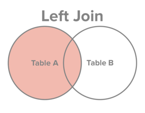
INNER JOIN or JOIN: retain just the rows each table that match the condition
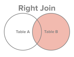
LEFT OUTER JOIN or LEFT JOIN: retain all rows in the first table, and just the rows in the second table that match the condition
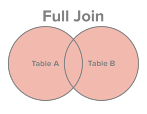
RIGHT OUTER JOIN or RIGHT JOIN: retain just the rows in the first table that match the condition, and all rows in the second table
FULL OUTER JOIN or FULL JOIN: retain all rows in both tables

Fields that cannot be filled in are assigned NA values

It helps to visualize the join types:

Examples

Suppose we want to figure out the average salaries of the players with the top 10 highest homerun averages. Then we’d have to combine the two tables below

dbGetQuery(con, paste("SELECT yearID, teamID, lgID, playerID, HR",
                      "FROM Batting", 
                      "ORDER BY playerID",
                      "LIMIT 10"))

##    yearID teamID lgID  playerID HR
## 1    2004    SFN   NL aardsda01  0
## 2    2006    CHN   NL aardsda01  0
## 3    2007    CHA   AL aardsda01  0
## 4    2008    BOS   AL aardsda01  0
## 5    2009    SEA   AL aardsda01  0
## 6    2010    SEA   AL aardsda01  0
## 7    2012    NYA   AL aardsda01  0
## 8    2013    NYN   NL aardsda01  0
## 9    2015    ATL   NL aardsda01  0
## 10   1954    ML1   NL aaronha01 13

dbGetQuery(con, paste("SELECT *",
                      "FROM Salaries",
                      "ORDER BY playerID",
                      "LIMIT 10"))

##    yearID teamID lgID  playerID  salary
## 1    2004    SFN   NL aardsda01  300000
## 2    2007    CHA   AL aardsda01  387500
## 3    2008    BOS   AL aardsda01  403250
## 4    2009    SEA   AL aardsda01  419000
## 5    2010    SEA   AL aardsda01 2750000
## 6    2011    SEA   AL aardsda01 4500000
## 7    2012    NYA   AL aardsda01  500000
## 8    1986    BAL   AL  aasedo01  600000
## 9    1987    BAL   AL  aasedo01  625000
## 10   1988    BAL   AL  aasedo01  675000

We can use a JOIN on the pair: yearID, playerID

dbGetQuery(con, paste("SELECT yearID, playerID, salary, HR",
                      "FROM Batting JOIN Salaries USING(yearID, playerID)",
                      "ORDER BY playerID",
                      "LIMIT 10"))

##    yearID  playerID  salary HR
## 1    2004 aardsda01  300000  0
## 2    2007 aardsda01  387500  0
## 3    2008 aardsda01  403250  0
## 4    2009 aardsda01  419000  0
## 5    2010 aardsda01 2750000  0
## 6    2012 aardsda01  500000  0
## 7    1986  aasedo01  600000  0
## 8    1987  aasedo01  625000  0
## 9    1988  aasedo01  675000  0
## 10   1989  aasedo01  400000  0

Note that here we’re missing 3 David Aardsma’s records (i.e., the JOIN discarded 3 records)

We can replicate this using merge() on imported data frames:

batting = dbReadTable(con, "Batting") 
salaries = dbReadTable(con, "Salaries") 
merged = merge(x=batting, y=salaries, by.x=c("yearID","playerID"), 
               by.y=c("yearID","playerID"))
merged[order(merged$playerID)[1:10], 
       c("yearID", "playerID", "salary", "HR")]

##       yearID  playerID  salary HR
## 16701   2004 aardsda01  300000  0
## 19371   2007 aardsda01  387500  0
## 20270   2008 aardsda01  403250  0
## 21157   2009 aardsda01  419000  0
## 22037   2010 aardsda01 2750000  0
## 23795   2012 aardsda01  500000  0
## 578     1986  aasedo01  600000  0
## 1353    1987  aasedo01  625000  0
## 2026    1988  aasedo01  675000  0
## 2733    1989  aasedo01  400000  0

For demonstration purposes, we can use a LEFT JOIN on the pair: yearID, playerID

dbGetQuery(con, paste("SELECT yearID, playerID, salary, HR",
                      "FROM Batting LEFT JOIN Salaries USING(yearID, playerID)",
                      "ORDER BY playerID",
                      "LIMIT 10"))

##    yearID  playerID  salary HR
## 1    2004 aardsda01  300000  0
## 2    2006 aardsda01      NA  0
## 3    2007 aardsda01  387500  0
## 4    2008 aardsda01  403250  0
## 5    2009 aardsda01  419000  0
## 6    2010 aardsda01 2750000  0
## 7    2012 aardsda01  500000  0
## 8    2013 aardsda01      NA  0
## 9    2015 aardsda01      NA  0
## 10   1954 aaronha01      NA 13

Now we can see that we have all 9 of David Aardsma’s original records from the Batting table (i.e., the LEFT JOIN kept them all, and just filled in an NA value when it was missing his salary)

Currently, RIGHT JOIN and FULL JOIN are not implemented in the RSQLite package

Now, as to our original question (average salaries of the players with the top 10 highest homerun averages):

dbGetQuery(con, paste("SELECT playerID, AVG(HR), AVG(salary)",
                      "FROM Batting JOIN Salaries USING(yearID, playerID)",
                      "GROUP BY playerID",
                      "ORDER BY Avg(HR) DESC",
                      "LIMIT 10"))

##     playerID  AVG(HR) AVG(salary)
## 1  bryankr01 39.00000      652000
## 2  pujolal01 36.93750    12752527
## 3  bondsba01 34.63636     8556606
## 4  mcgwima01 34.29412     4814021
## 5  arenano01 33.66667     2004167
## 6  howarry01 33.30000    15525500
## 7  troutmi01 33.25000     5919083
## 8  duvalad01 33.00000      510000
## 9  cartech02 32.75000     1919750
## 10 kingmda01 32.50000      908750

Summary

R jargon	Database jargon	Tidyverse
column	field
row	record
data frame	table
types of the columns	table schema
collection of data frames	database
conditional indexing	`SELECT`, `FROM`, `WHERE`, `HAVING`	`dplyr::select()`, `dplyr::filter()`
`tapply()` or other means	`GROUP BY`	`dplyr::group_by()`
`order()`	`ORDER BY`	`dplyr::arrange()`
`merge()`	`INNER JOIN` or just `JOIN`	`tidyr::inner_join()`

Relational Databases

Last week: Debugging

Part I

What is a database?

Databases versus data frames

Why do we need database software?

Client-server model and SQL

Connecting R to SQLite

Listing what’s available

Importing a table as a data frame

SELECT

Examples

ORDER BY

Part II

SELECT, expanded

Examples

GROUP BY

AS

WHERE

HAVING

Part III

SELECT, expanded

JOIN

Examples

Summary

`SELECT`

`ORDER BY`

`SELECT`, expanded

`GROUP BY`

`AS`

`WHERE`

`HAVING`

`SELECT`, expanded

`JOIN`