Why statisticians learn to program

Coding is an essential, integral component of data analysis: coding, along with basic knowledge of statistical principles and methods, has become a basic form of modern-day literacy, not just in scientific and academic circles, but in real life. It is extremely likely (nearly certain) that, at your next job interview, you will need to demonstrate adequate coding skills and that coding will be an integral part of your job as a statistician/data scientist, whatever that may be. In addition to R, consider learning other languages: Pyhton for data science and julia for scientific computing.
Independence: otherwise, you rely on someone else giving you exactly the right tool.
Honesty: otherwise, you end up distorting your problem to match the tools you have.
Reproducibility: make your code public so that others can replicate your anakysis and arrive at the same finding.
Clarity: often, turning your ideas into something a machine can do refines your thinking.

Cool example: shiny documents

Shiny is a R package that allows to write interactive web applications. Check out the Shiny Gallery

Cool example: catching an intruder

This is a very nice problem suggested as an example by Prof. Ryan Tibshirani.

Assume a $n \times n$ grid of empty squares, with an intruder hiding behind a square, unknown to us. At each time point:

the intruder will randomly choose to stay put or to move to any of the the adjacent squares (up, down, left or right, if applicable);
we scan all the $n^2$ squares simultaneously using a faulty device: if a square hides the intruder the device will correctly indicate so, but if the square is empty the device will incorrectly report that it is occupied with probability $p \in [0,1]$, independently across squares and across times.

Our goal is to locate the intruder. Notice that, as times goes by, using brute force we are able to dynamically maintain a list of potential locations for the intruder, with the size of the list fluctuating over time. (Coding exercise: how would create and update such list?)

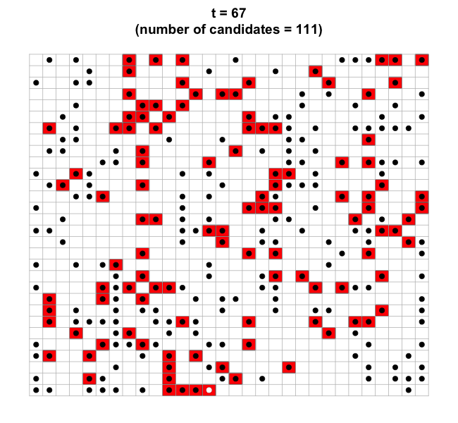
There are several questions we could ask:

will this list eventually shrink in size to reduce to only one entry, which will identify the location of the intruder?
how long would this process take?
what is the impact of the grid size parameter $n$ and of the probability parameter $p$ on the probability of eventually catching the intruder and on the amount of time (number of time steps) before this happens?
is there a better (more efficient and/or more accurate) algorithm than the natural one described above?

We can deploy simulations to attempt to tackle the above questions. Absent any theoretical answers (which, to the best of my knowledge, have not been worked out yet), that is the best we can do. Take a look at the R code used for simulations, written by Prof. Ryan Tibshirani. By the end of this course (in fact, hopefully sooner) you should be able to read and understand it.

source("https://www.stat.cmu.edu/~arinaldo/Teaching/36350/F22/lectures/intruder.R")
intruder.sim(n=30, p=0.1)

## [1] 7

#intruder.sim(n=50, p=0.2, dt=0.1)
#intruder.sim(n=50, p=0.3, dt=0.1)

Part I

Data types, operators, variables

This class in a nutshell: functional programming

Two basic types of things/objects: data and functions

Data: things like 7, “seven”, $7.000$, and $\left[ \begin{array}{ccc} 7 & 7 & 7 \\ 7 & 7 & 7\end{array}\right]$
Functions: things like log, + (takes two arguments), < (two), %% (two), and mean (one)

A function is a machine which turns input objects, or arguments, into an output object, or a return value (possibly with side effects), according to a definite rule

Programming is writing functions to transform inputs (other functions or data) into outputs
Good programming ensures the transformation is done easily and correctly
Machines are made out of machines; functions are made out of functions, like $f(a,b) = a^2 + b^2$

The trick to good programming is to take a big transformation and break it down into smaller ones, and then break those down, until you come to tasks which are easy (using built-in functions)

Before functions, data

At base level, all data can represented in binary format, by bits (i.e., TRUE/FALSE, YES/NO, 1/0). Basic data types:

Booleans: Direct binary values: TRUE or FALSE in R
Integers: whole numbers (positive, negative or zero), represented by a fixed-length block of bits
Characters: fixed-length blocks of bits, with special coding; strings: sequences of characters
Floating point numbers: an integer times a positive integer to the power of an integer, as in $3 \times 10^6$ or $1 \times 3^{-1}$
Missing or ill-defined values: NA, NaN, etc.

Operators

Unary: take just one argument. E.g., - for arithmetic negation, ! for Boolean negation
Binary: take two arguments. E.g., +, -, *, and / (though this is only a partial operator). Also, %% (for mod), and ^ (again partial)

-7

## [1] -7

7 + 5

## [1] 12

7 - 5

## [1] 2

7 * 5

## [1] 35

7 ^ 5

## [1] 16807

7 / 5

## [1] 1.4

7 %% 5

## [1] 2

Comparison operators

These are also binary operators; they take two objects, and give back a Boolean

7 > 5

## [1] TRUE

7 < 5

## [1] FALSE

7 >= 7

## [1] TRUE

7 <= 5

## [1] FALSE

7 == 5

## [1] FALSE

7 != 5

## [1] TRUE

Warning: == is a comparison operator, = is not!

Logical operators

These basic ones are & (and) and | (or)

(5 > 7) & (6 * 7 == 42)

## [1] FALSE

(5 > 7) | (6 * 7 == 42)

## [1] TRUE

(5 > 7) | (6 * 7 == 42) & (0 != 0)

## [1] FALSE

(5 > 7) | (6 * 7 == 42) & (0 != 0) | (9 - 8 >= 0)

## [1] TRUE

Note: The double forms && and || are different! We’ll see them later

More types

The typeof() function returns the data type
is.foo() functions return Booleans for whether the argument is of type foo
as.foo() (tries to) “cast” its argument to type foo, to translate it sensibly into such a value

typeof(7)

## [1] "double"

is.numeric(7)

## [1] TRUE

is.na(7)

## [1] FALSE

is.na(7/0)

## [1] FALSE

is.na(0/0)

## [1] TRUE

is.character(7)

## [1] FALSE

is.character("7")

## [1] TRUE

is.character("seven")

## [1] TRUE

is.na("seven")

## [1] FALSE

as.character(5/6)

## [1] "0.833333333333333"

as.numeric(as.character(5/6))

## [1] 0.8333333

6 * as.numeric(as.character(5/6))

## [1] 5

5/6 == as.numeric(as.character(5/6))

## [1] FALSE

Data can have names

We can give names to data objects; these give us variables. Some variables are built-in:

pi

## [1] 3.141593

Variables can be arguments to functions or operators, just like constants:

pi * 10

## [1] 31.41593

cos(pi)

## [1] -1

We create variables with the assignment operator, <- or =

approx.pi = 22/7
approx.pi

## [1] 3.142857

diameter = 10
approx.pi * diameter

## [1] 31.42857

The assignment operator also changes values:

circumference = approx.pi * diameter
circumference

## [1] 31.42857

circumference = 30
circumference

## [1] 30

The code you write will be made of variables, with descriptive names
Easier to design, easier to debug, easier to improve, and easier for others to read
Avoid “magic constants”; instead use named variables
Named variables are a first step towards abstraction

R workspace

What variables have you defined?

ls()

## [1] "approx.pi"     "circumference" "diameter"

Getting rid of variables:

rm("circumference")
ls()

## [1] "approx.pi" "diameter"

rm(list=ls()) # Be warned! This erases everything
ls()

## character(0)

Part II

Data structures

First data structure: vectors

A data structure is a grouping of related data values into an object
A vector is a sequence of values, all of the same type

x = c(7, 8, 10, 45)
x

## [1]  7  8 10 45

is.vector(x)

## [1] TRUE

The c() function returns a vector containing all its arguments in specified order
1:5 is shorthand for c(1,2,3,4,5), and so on
x[1] would be the first element, x[4] the fourth element, and x[-4] is a vector containing all but the fourth element

vector(length=n) returns an empty vector of length n; helpful for filling things up later

weekly.hours = vector(length=5)
weekly.hours

## [1] FALSE FALSE FALSE FALSE FALSE

weekly.hours[5] = 8
weekly.hours

## [1] 0 0 0 0 8

Vector arithmetic

Arithmetic operator apply to vectors in a “componentwise” fashion

y = c(-7, -8, -10, -45)
x + y

## [1] 0 0 0 0

x * y

## [1]   -49   -64  -100 -2025

Recycling

Recycling repeat elements in shorter vector when combined with a longer one

x + c(-7,-8)

## [1]  0  0  3 37

x^c(1,0,-1,0.5)

## [1] 7.000000 1.000000 0.100000 6.708204

Single numbers are vectors of length 1 for purposes of recycling:

2 * x

## [1] 14 16 20 90

Can do componentwise comparisons with vectors:

x > 9

## [1] FALSE FALSE  TRUE  TRUE

Logical operators also work elementwise:

(x > 9) & (x < 20)

## [1] FALSE FALSE  TRUE FALSE

To compare whole vectors, best to use identical() or all.equal():

x == -y

## [1] TRUE TRUE TRUE TRUE

identical(x, -y)

## [1] TRUE

identical(c(0.5-0.3,0.3-0.1), c(0.3-0.1,0.5-0.3))

## [1] FALSE

all.equal(c(0.5-0.3,0.3-0.1), c(0.3-0.1,0.5-0.3))

## [1] TRUE

Note: these functions are slightly different; we’ll see more later

Functions on vectors

Many functions can take vectors as arguments:

mean(), median(), sd(), var(), max(), min(), length(), and sum() return single numbers
sort() returns a new vector
hist() takes a vector of numbers and produces a histogram, a highly structured object, with the side effect of making a plot
ecdf() similarly produces a cumulative-density-function object
summary() gives a five-number summary of numerical vectors
any() and all() are useful on Boolean vectors

Indexing vectors

Vector of indices:

x[c(2,4)]

## [1]  8 45

Vector of negative indices:

x[c(-1,-3)]

## [1]  8 45

Boolean vector:

x[x > 9]

## [1] 10 45

y[x > 9]

## [1] -10 -45

which() gives the elements of a Boolean vector that are TRUE:

places = which(x > 9)
places

## [1] 3 4

y[places]

## [1] -10 -45

Named components

We can give names to elements/components of vectors, and index vectors accordingly

names(x) = c("v1","v2","v3","fred")
names(x)

## [1] "v1"   "v2"   "v3"   "fred"

x[c("fred","v1")]

## fred   v1 
##   45    7

Note: here R is printing the labels, these are not additional components of x

names() returns another vector (of characters):

names(y) = names(x)
sort(names(x))

## [1] "fred" "v1"   "v2"   "v3"

which(names(x) == "fred")

## [1] 4

Second data structure: arrays

An array is a multi-dimensional generalization of vectors

x = c(7, 8, 10, 45)
x.arr = array(x, dim=c(2,2))
x.arr

##      [,1] [,2]
## [1,]    7   10
## [2,]    8   45

dim says how many rows and columns; filled by columns
Can have 3d arrays, 4d arrays, etc.; dim is vector of arbitrary length

Some properties of our array:

dim(x.arr)

## [1] 2 2

is.vector(x.arr)

## [1] FALSE

is.array(x.arr)

## [1] TRUE

typeof(x.arr)

## [1] "double"

Indexing arrays

Can access a 2d array either by pairs of indices or by the underlying vector (column-major order):

x.arr[1,2]

## [1] 10

x.arr[3]

## [1] 10

Omitting an index means “all of it”:

x.arr[c(1,2),2]

## [1] 10 45

x.arr[,2]

## [1] 10 45

x.arr[,2,drop=FALSE]

##      [,1]
## [1,]   10
## [2,]   45

Note: the optional third argument drop=FALSE ensures that the result is still an array, not a vector

Functions on arrays

Many functions applied to an array will just boil things down to the underlying vector:

which(x.arr > 9)

## [1] 3 4

This happens unless the function is set up to handle arrays specifically

And there are several functions/operators that do preserve array structure:

y = -x
y.arr = array(y, dim=c(2,2))
y.arr + x.arr

##      [,1] [,2]
## [1,]    0    0
## [2,]    0    0

2d arrays: matrices

A matrix is a specialization of a 2d array

z.mat = matrix(c(40,1,60,3), nrow=2)
z.mat

##      [,1] [,2]
## [1,]   40   60
## [2,]    1    3

is.array(z.mat)

## [1] TRUE

is.matrix(z.mat)

## [1] TRUE

Could also specify ncol for the number of columns
To fill by rows, use byrow=TRUE
Elementwise operations with the usual arithmetic and comparison operators (e.g., z.mat/3)

Matrix multiplication

Matrices have its own special multiplication operator, written %*%:

six.sevens = matrix(rep(7,6), ncol=3)
six.sevens

##      [,1] [,2] [,3]
## [1,]    7    7    7
## [2,]    7    7    7

z.mat %*% six.sevens # [2x2] * [2x3]

##      [,1] [,2] [,3]
## [1,]  700  700  700
## [2,]   28   28   28

Can also multiply a matrix and a vector

Row/column manipulations

Row/column sums, or row/column means:

rowSums(z.mat)

## [1] 100   4

colSums(z.mat)

## [1] 41 63

rowMeans(z.mat)

## [1] 50  2

colMeans(z.mat)

## [1] 20.5 31.5

Matrix diagonal

The diag() function can be used to extract the diagonal entries of a matrix:

diag(z.mat)

## [1] 40  3

It can also be used to change the diagonal:

diag(z.mat) = c(35,4)
z.mat

##      [,1] [,2]
## [1,]   35   60
## [2,]    1    4

Creating a diagonal matrix

Finally, diag() can be used to create a diagonal matrix:

diag(c(3,4))

##      [,1] [,2]
## [1,]    3    0
## [2,]    0    4

diag(2)

##      [,1] [,2]
## [1,]    1    0
## [2,]    0    1

Other matrix operators

Transpose:

t(z.mat)

##      [,1] [,2]
## [1,]   35    1
## [2,]   60    4

Determinant:

det(z.mat)

## [1] 80

Inverse:

solve(z.mat)

##         [,1]    [,2]
## [1,]  0.0500 -0.7500
## [2,] -0.0125  0.4375

z.mat %*% solve(z.mat)

##      [,1] [,2]
## [1,]    1    0
## [2,]    0    1

Names in matrices

We can name either rows or columns or both, with rownames() and colnames()
These are just character vectors, and we use them just like we do names() for vectors
Names help us understand what we’re working with

Third data structure: lists

A list is sequence of values, but not necessarily all of the same type

my.dist = list("exponential", 7, FALSE)
my.dist

## [[1]]
## [1] "exponential"
## 
## [[2]]
## [1] 7
## 
## [[3]]
## [1] FALSE

Most of what you can do with vectors you can also do with lists

Accessing pieces of lists

Can use [ ] as with vectors
Or use [[ ]], but only with a single index [[ ]] drops names and structures, [ ] does not

my.dist[2]

## [[1]]
## [1] 7

my.dist[[2]]

## [1] 7

my.dist[[2]]^2

## [1] 49

Expanding and contracting lists

Add to lists with c() (also works with vectors):

my.dist = c(my.dist, 9)
my.dist

## [[1]]
## [1] "exponential"
## 
## [[2]]
## [1] 7
## 
## [[3]]
## [1] FALSE
## 
## [[4]]
## [1] 9

Chop off the end of a list by setting the length to something smaller (also works with vectors):

length(my.dist)

## [1] 4

length(my.dist) = 3
my.dist

## [[1]]
## [1] "exponential"
## 
## [[2]]
## [1] 7
## 
## [[3]]
## [1] FALSE

Pluck out all but one piece of a list (also works with vectors):

my.dist[-2]

## [[1]]
## [1] "exponential"
## 
## [[2]]
## [1] FALSE

Names in lists

We can name some or all of the elements of a list:

names(my.dist) = c("family","mean","is.symmetric")
my.dist

## $family
## [1] "exponential"
## 
## $mean
## [1] 7
## 
## $is.symmetric
## [1] FALSE

my.dist[["family"]]

## [1] "exponential"

my.dist["family"]

## $family
## [1] "exponential"

Lists have a special shortcut way of using names, with $:

my.dist[["family"]]

## [1] "exponential"

my.dist$family

## [1] "exponential"

Creating a list with names:

another.dist = list(family="gaussian", mean=7, sd=1, is.symmetric=TRUE)

Adding named elements:

my.dist$was.estimated = FALSE
my.dist[["last.updated"]] = "2021-01-01"

Removing a named list element, by assigning it the value NULL:

my.dist$was.estimated = NULL

Key-value pairs

Lists give us a natural way to store and look up data by name, rather than by position
A really useful programming concept with many names: key-value pairs, i.e., dictionaries, or associative arrays
If all our distributions have components named family, we can look that up by name, without caring where it is (in what position it lies) in the list

Data frames

The classic data table, $n$ rows for cases, $p$ columns for variables
Lots of the really-statistical parts of R presume data frames
Not just a matrix because columns can have different types
Many matrix functions also work for data frames (e.g.,rowSums(), summary(), apply())

a.mat = matrix(c(35,8,10,4), nrow=2)
colnames(a.mat) = c("v1","v2")
a.mat

##      v1 v2
## [1,] 35 10
## [2,]  8  4

a.mat[,"v1"]  # Try a.mat$v1 and see what happens

## [1] 35  8

a.df = data.frame(a.mat,logicals=c(TRUE,FALSE))
a.df

##   v1 v2 logicals
## 1 35 10     TRUE
## 2  8  4    FALSE

a.df$v1

## [1] 35  8

a.df[,"v1"]

## [1] 35  8

a.df[1,]

##   v1 v2 logicals
## 1 35 10     TRUE

colMeans(a.df)

##       v1       v2 logicals 
##     21.5      7.0      0.5

Adding rows and columns

We can add rows or columns to an array or data frame with rbind() and cbind(), but be careful about forced type conversions

rbind(a.df,list(v1=-3,v2=-5,logicals=TRUE))

##   v1 v2 logicals
## 1 35 10     TRUE
## 2  8  4    FALSE
## 3 -3 -5     TRUE

rbind(a.df,c(3,4,6))

##   v1 v2 logicals
## 1 35 10        1
## 2  8  4        0
## 3  3  4        6

Much more on data frames a bit later in the course …

Structures of structures

So far, every list element has been a single data value. List elements can be other data structures, e.g., vectors and matrices, even other lists:

my.list = list(z.mat=z.mat, my.lucky.num=13, my.dist=my.dist)
my.list

## $z.mat
##      [,1] [,2]
## [1,]   35   60
## [2,]    1    4
## 
## $my.lucky.num
## [1] 13
## 
## $my.dist
## $my.dist$family
## [1] "exponential"
## 
## $my.dist$mean
## [1] 7
## 
## $my.dist$is.symmetric
## [1] FALSE
## 
## $my.dist$last.updated
## [1] "2021-01-01"

Introduction and R Basics