Statistical Prediction
Statistical Computing, 36-350
Tuesday December 6, 2022
Part I
Training and testing errors
Reminder: statistical (regression) models
You have some data \(X_1,\ldots,X_p,Y\): the variables \(X_1,\ldots,X_p\) are called predictors, and \(Y\) is called a response. You’re interested in the relationship that governs them
So you posit that \(Y|X_1,\ldots,X_p \sim P_\theta\), where \(\theta\) represents some unknown parameters. This is called regression model for \(Y\) given \(X_1,\ldots,X_p\). Goal is to estimate parameters. Why?
- To assess model validity, predictor importance (inference)
- To predict future \(Y\)’s from future \(X_1,\ldots,X_p\)’s (prediction)
Reminder: linear regression models
The linear model is arguably the most widely used statistical model, has a place in nearly every application domain of statistics
Given response \(Y\) and predictors \(X_1,\ldots,X_p\), in a linear regression model, we posit:
\[ Y = \beta_0 + \beta_1 X_1 + \ldots + \beta_p X_p + \epsilon, \quad \text{where $\epsilon \sim N(0,\sigma^2)$} \]
Goal is to estimate parameters \(\beta_0,\beta_1,\ldots,\beta_p\). Why?
- To assess whether the linear model is true, which predictors are important (inference)
- To simply predict future \(Y\)’s from future \(X_1,\ldots,X_p\)’s (prediction)
Good diagnostics, or good predictions?
Nowadays, we try to fit linear models in such a wide variety of difficult problem settings that, in many cases, we have no reason to believe the true data generating model is linear, the errors are close to Gaussian or homoskedastic, etc. Hence, a modern perspective:
The linear model is only a rough approximation, so evaluate prediction accuracy, and let this determine its usefulness
This idea, to focus on prediction, is far more general than linear models. More on this, shortly
Test error
Suppose we have training data \(X_{i1},\ldots,X_{ip},Y_i\), \(i=1,\ldots,n\) used to estimate regression coefficients \(\hat{\beta}_0,\hat{\beta}_1,\ldots,\hat{\beta}_p\)
Given new \(X_1^*,\ldots,X_p^*\) and asked to predict the associated \(Y^*\). From the estimated linear model, prediction is: \(\hat{Y}^* = \hat{\beta}_0 + \hat{\beta}_1 X_1^* + \ldots + \hat{\beta}_p X_p^*\). We define the test error, also called prediction error, by \[ \mathbb{E}(Y^* - \hat{Y}^*)^2 \] where the expectation is over every random: training data, \(X_{i1},\ldots,X_{ip},Y_i\), \(i=1,\ldots,n\) and test data, \(X_1^*,\ldots,X_p^*,Y^*\)
This was explained for a linear model, but the same definition of test error holds in general
Estimating test error
Often, we want an accurate estimate of the test error of our method (e.g., linear regression). Why? Two main purposes:
Predictive assessment: get an absolute understanding of the magnitude of errors we should expect in making future predictions
Model/method selection: choose among different models/methods, attempting to minimize test error
Training error
Suppose, as an estimate the test error of our method, we take the observed training error \[ \frac{1}{n} \sum_{i=1}^n (Y_i - \hat{Y}_i)^2 \]
What’s wrong with this? Generally too optimistic as an estimate of the test error—after all, the parameters \(\hat{\beta}_0,\hat{\beta}_1,,\ldots,\hat{\beta}_p\) were estimated to make \(\hat{Y}_i\) close to \(Y_i\), \(i=1,\ldots,n\), in the first place!
Also, importantly, the more complex/adaptive the method, the more optimistic its training error is as an estimate of test error
Examples
set.seed(1)
n = 30
x = sort(runif(n, -3, 3))
y = 2*x + 2*rnorm(n)
x0 = sort(runif(n, -3, 3))
y0 = 2*x0 + 2*rnorm(n)

par(mfrow=c(1,2))
xlim = range(c(x,x0)); ylim = range(c(y,y0))
plot(x, y, xlim=xlim, ylim=ylim, main="Training data")
plot(x0, y0, xlim=xlim, ylim=ylim, main="Test data")
# Training and test errors for a simple linear model
lm.1 = lm(y ~ x)
yhat.1 = predict(lm.1, data.frame(x=x))
train.err.1 = mean((y-yhat.1)^2)
y0hat.1 = predict(lm.1, data.frame(x=x0))
test.err.1 = mean((y0-y0hat.1)^2)
par(mfrow=c(1,2))
plot(x, y, xlim=xlim, ylim=ylim, main="Training data")
lines(x, yhat.1, col=2, lwd=2)
text(0, -6, label=paste("Training error:", round(train.err.1,3)))
plot(x0, y0, xlim=xlim, ylim=ylim, main="Test data")
lines(x0, y0hat.1, col=3, lwd=2)
text(0, -6, label=paste("Test error:", round(test.err.1,3)))# Training and test errors for a 10th order polynomial regression
# (The problem is only exacerbated!)
lm.10 = lm(y ~ poly(x,10))
yhat.10 = predict(lm.10, data.frame(x=x))
train.err.10 = mean((y-yhat.10)^2)
y0hat.10 = predict(lm.10, data.frame(x=x0))
test.err.10 = mean((y0-y0hat.10)^2)
par(mfrow=c(1,2))
xx = seq(min(xlim), max(xlim), length=100)
plot(x, y, xlim=xlim, ylim=ylim, main="Training data")
lines(xx, predict(lm.10, data.frame(x=xx)), col=2, lwd=2)
text(0, -6, label=paste("Training error:", round(train.err.10,3)))
plot(x0, y0, xlim=xlim, ylim=ylim, main="Test data")
lines(xx, predict(lm.10, data.frame(x=xx)), col=3, lwd=2)
text(0, -6, label=paste("Test error:", round(test.err.10,3)))Part II
Sample-splitting and cross-validation
Sample-splitting
Given a data set, how can we estimate test error? (Can’t simply simulate more data for testing.) We know training error won’t work
A tried-and-true technique with an old history in statistics: sample-splitting
- Split the data set into two parts
- First part: train the model/method
- Second part: make predictions
- Evaluate observed test error
Examples
dat = read.table("https://www.stat.cmu.edu/~arinaldo/Teaching/36350/F22/data/xy.dat")
head(dat)
n = nrow(dat)
# Split data in half, randomly
set.seed(0)
inds = sample(rep(1:2, length=n))
head(inds, 10)## [1] 2 2 1 1 2 1 1 2 2 1table(inds)## inds
## 1 2
## 25 25dat.tr = dat[inds==1,] # Training data
dat.te = dat[inds==2,] # Test data
plot(dat$x, dat$y, pch=c(21,19)[inds], main="Sample-splitting")
legend("topleft", legend=c("Training","Test"), pch=c(21,19))# Train on the first half
lm.1 = lm(y ~ x, data=dat.tr)
lm.10 = lm(y ~ poly(x,10), data=dat.tr)
# Predict on the second half, evaluate test error
pred.1 = predict(lm.1, data.frame(x=dat.te$x))
pred.10 = predict(lm.10, data.frame(x=dat.te$x))
test.err.1 = mean((dat.te$y - pred.1)^2)
test.err.10 = mean((dat.te$y - pred.10)^2)
# Plot the results
par(mfrow=c(1,2))
xx = seq(min(dat$x), max(dat$x), length=100)
plot(dat$x, dat$y, pch=c(21,19)[inds], main="Sample-splitting")
lines(xx, predict(lm.1, data.frame(x=xx)), col=2, lwd=2)
legend("topleft", legend=c("Training","Test"), pch=c(21,19))
text(0, -6, label=paste("Test error:", round(test.err.1,3)))
plot(dat$x, dat$y, pch=c(21,19)[inds], main="Sample-splitting")
lines(xx, predict(lm.10, data.frame(x=xx)), col=3, lwd=2)
legend("topleft", legend=c("Training","Test"), pch=c(21,19))
text(0, -6, label=paste("Test error:", round(test.err.10,3)))Cross-validation
Sample-splitting is simple, effective. But its it estimates the test error when the model/method is trained on less data (say, roughly half as much)
An improvement over sample splitting: \(k\)-fold cross-validation
- Split data into \(k\) parts or folds
- Use all but one fold to train your model/method
- Use the left out folds to make predictions
- Rotate around the roles of folds, \(k\) rounds total
- Compute squared error of all predictions, in the end
A common choice is \(k=5\) or \(k=10\) (sometimes \(k=n\), called leave-one-out!)

For demonstration purposes, suppose \(n=6\) and we choose \(k=3\) parts
| Data point | Part | Trained on | Prediction |
|---|---|---|---|
| \(Y_1\) | 1 | 2,3 | \(\hat{Y}^{-(1)}_1\) |
| \(Y_2\) | 1 | 2,3 | \(\hat{Y}^{-(1)}_2\) |
| \(Y_3\) | 2 | 1,3 | \(\hat{Y}^{-(2)}_3\) |
| \(Y_4\) | 2 | 1,3 | \(\hat{Y}^{-(2)}_4\) |
| \(Y_5\) | 3 | 1,2 | \(\hat{Y}^{-(3)}_5\) |
| \(Y_6\) | 3 | 1,2 | \(\hat{Y}^{-(3)}_6\) |
Notation: model trained on parts 2 and 3 in order to make predictions for part 1. So prediction \(\hat{Y}^{-(1)}_1\) for \(Y_1\) comes from model trained on all data except that in part 1. And so on
The cross-validation estimate of test error (also called the cross-validation error) is \[ \frac{1}{6}\Big( (Y_1-\hat{Y}^{-(1)}_1)^2 + (Y_2-\hat{Y}^{-(1)}_2)^2 + (Y_3-\hat{Y}^{-(2)}_3)^2 + \\ (Y_4-\hat{Y}^{-(2)}_4)^2 + (Y_5-\hat{Y}^{-(3)}_5)^2 + (Y_6-\hat{Y}^{-(3)}_6)^2 \Big) \]
Examples
# Split data in 5 parts, randomly
k = 5
set.seed(0)
inds = sample(rep(1:k, length=n))
head(inds, 10)
## [1] 4 4 4 1 4 3 3 5 3 3table(inds)## inds
## 1 2 3 4 5
## 10 10 10 10 10# Now run cross-validation: easiest with for loop, running over
# which part to leave out
pred.mat = matrix(0, n, 2) # Empty matrix to store predictions
for (i in 1:k) {
cat(paste("Fold",i,"... "))
dat.tr = dat[inds!=i,] # Training data
dat.te = dat[inds==i,] # Test data
# Train our models
lm.1.minus.i = lm(y ~ x, data=dat.tr)
lm.10.minus.i = lm(y ~ poly(x,10), data=dat.tr)
# Record predictions
pred.mat[inds==i,1] = predict(lm.1.minus.i, data.frame(x=dat.te$x))
pred.mat[inds==i,2] = predict(lm.10.minus.i, data.frame(x=dat.te$x))
}## Fold 1 ... Fold 2 ... Fold 3 ... Fold 4 ... Fold 5 ...# Compute cross-validation error, one for each model
cv.errs = colMeans((pred.mat - dat$y)^2)
# Plot the results
par(mfrow=c(1,2))
xx = seq(min(dat$x), max(dat$x), length=100)
plot(dat$x, dat$y, pch=20, col=inds+1, main="Cross-validation")
lines(xx, predict(lm.1, data.frame(x=xx)), # Note: model trained on FULL data!
lwd=2, lty=2)
legend("topleft", legend=paste("Fold",1:k), pch=20, col=2:(k+1))
text(0, -6, label=paste("CV error:", round(cv.errs[1],3)))
plot(dat$x, dat$y, pch=20, col=inds+1, main="Cross-validation")
lines(xx, predict(lm.10, data.frame(x=xx)), # Note: model trained on FULL data!
lwd=2, lty=2)
legend("topleft", legend=paste("Fold",1:k), pch=20, col=2:(k+1))
text(0, -6, label=paste("CV error:", round(cv.errs[2],3)))# Now we visualize the different models trained, one for each CV fold
for (i in 1:k) {
dat.tr = dat[inds!=i,] # Training data
dat.te = dat[inds==i,] # Test data
# Train our models
lm.1.minus.i = lm(y ~ x, data=dat.tr)
lm.10.minus.i = lm(y ~ poly(x,10), data=dat.tr)
# Plot fitted models
par(mfrow=c(1,2)); cols = c("red","gray")
plot(dat$x, dat$y, pch=20, col=cols[(inds!=i)+1], main=paste("Fold",i))
lines(xx, predict(lm.1.minus.i, data.frame(x=xx)), lwd=2, lty=2)
legend("topleft", legend=c(paste("Fold",i),"Other folds"), pch=20, col=cols)
text(0, -6, label=paste("Fold",i,"error:",
round(mean((dat.te$y - pred.mat[inds==i,1])^2),3)))
plot(dat$x, dat$y, pch=20, col=cols[(inds!=i)+1], main=paste("Fold",i))
lines(xx, predict(lm.10.minus.i, data.frame(x=xx)), lwd=2, lty=2)
legend("topleft", legend=c(paste("Fold",i),"Other folds"), pch=20, col=cols)
text(0, -6, label=paste("Fold",i,"error:",
round(mean((dat.te$y - pred.mat[inds==i,2])^2),3)))
}Part III
Statistical prediction
Shifting tides: a focus on prediction
Classically, statistics has focused in large part on inference. The tides are shifting (at least in some part), and in many modern problems, the following view is taken:
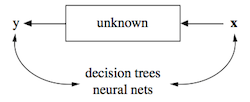
Models are only approximations; some methods need not even have underlying models; let’s evaluate prediction accuracy, and let this determine model/method usefulness
This is (in some sense) one of the basic tenets of machine learning
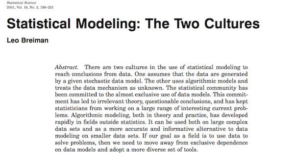
“Early” influential paper
 versus
  ?
?
Statistical prediction machines
Some methods for predicting \(Y\) from \(X_1,\ldots,X_p\) have (in a sense) no parameters at all. Perhaps better said: they are not motivated from writing down a statistical model like \(Y|X_1,\ldots,X_p \sim P_\theta\)
We’ll call these statistical prediction machines. Admittedly: not a real term, but it’s evocative of what they are doing, and there’s no real consensus terminology. You might also see these described as:
- Model-free methods
- Distribution-free methods
- Machine learning methods
Comment: in a broad sense, most of these methods would have been completely unthinkable before the rise of high-performance computing
\(k\)-nearest neighbors
One of the simplest prediction machines: \(k\)-nearest neighbors regression
- Given training data \(X_i=(X_{i1},\ldots,X_{ip})\) and \(Y_i\), \(i=1,\ldots,n\)
- Given a new test point \(X^*=(X^*_1,\ldots,X^*_p)\)
- Find \(k\)-nearest training points \(X_{(1)},\ldots,X_{(k)}\) to \(X^*\)
- Use as our prediction \(\hat{Y}^*=\sum_{i=1}^k Y_{(i)}/k\)
Ask yourself: what happens when \(k=1\)? What happens when \(k=n\)?
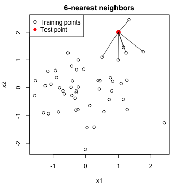
Advantages: simple and flexible. Disadvantages: can be slow and cumbersome
From \(k\)-nearest neighbors to trees
Can think of 1-nearest neighbor predictions as being simply given by predicting a constant within each element of what is called as Voronoi tesellation: these are polyhedra that partition the predictor space

Regression trees are similar but somewhat different. In a nutshell, they use (nested) rectangles instead of polyhedra. These rectangles are fit through sequential (greedy) split-point determinations
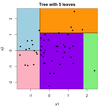
Advantage: easier to make predictions (from split-points). Disadvantage: less flexible
From trees to boosting
Boosting is a method built on top of regression trees in a clever way. To make predictions, can think of taking predictions from a sequence of trees, and combining them with weights (coefficients)
\(\beta_1 \cdot\) 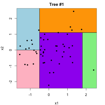 \(+\) \(\beta_2 \cdot\)
 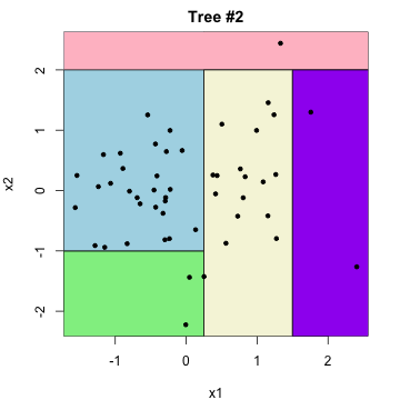 \(+\ldots\)
Advantage: much more flexible than a single tree. Disadvantage: not generally interpretable …
Many, many others
There are many, many other statistical prediction methods out there; examples below. If you’re interesting in learning more, take 36-462 Data Mining, or one of the Introduction to Machine Learning Courses 10-401, 10-601, 10-701
- Kernel machines
- Random forests
- Random projections
- Neural networks
- etc.
Two world views?
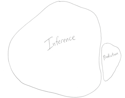 versus
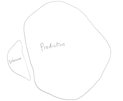
Conclusion
- Neither view is completely right, of course
- Inference, prediction are still both extremely important in their own right
- And even still, there is much more to statistics than these two
- Best you can do: be well-informed about all of your modeling options
- Also be well-informed about how you can fit them and assess them!